In Excel 2013, fix the line or columns and color to make it easier to see the display

I want to check the data in the list format, but it may be difficult to see because there are too many items.This time, let's introduce a technique that makes it easier to see the list by making full use of the color coding of “row and column fixation” and “conditional format”.

■ If you use an Excel that makes it easy to see the display of rows and columns, it may be difficult to check because the necessary items and items are too separated.Therefore, what I want to use is “fixing rows and columns”.Since the row of the item name and the column of the name can be fixed, the remaining part can be scrolled, making it easier to check the value.

It is also effective to change the color by changing the color for each row or column.If you use the “conditional format”, you can automatically color the rows and columns that apply to the conditions, and you can immediately find the applicable members and items without checking the data in detail.

■ Fix rows and columns

↑ Select the cell on the right side of the column you want to fix (in the case of rows, one lower), and select “Fix the window frame” on the “Display” tab.

↑ The first line is fixed, and the second line scrolls.

↑ You can see that the column B is scrolling.

↑ If you only need to fix the first line or the first column, there is a special menu.It is lactin that you do not have to choose cells one by one.

↑ It is also possible to make multiple rows and columns to be fixed.The number of columns and lines that can be fixed is not particularly limited and can be changed as needed.

■ Conditional format that automatically colored in a conditional format is characterized by determining a specific keyword or numerical value, and when the corresponding value is entered in the cell, it can be changed immediately to the format that has been set in advance.is.You can also set multiple format rules, and it is extremely useful when the input data is classified by genre.

STEP1 Calling the management window of the format rule

↑ Specify the entire table, select a “conditional format” on the “home” tab, and select “Rule management” from the displayed menu.

↑ The management window of the formula rule is displayed.If you select the "new rule" button in the upper left, you can create a new conditional format.

Step2 The search target and the corresponding cell format are determined

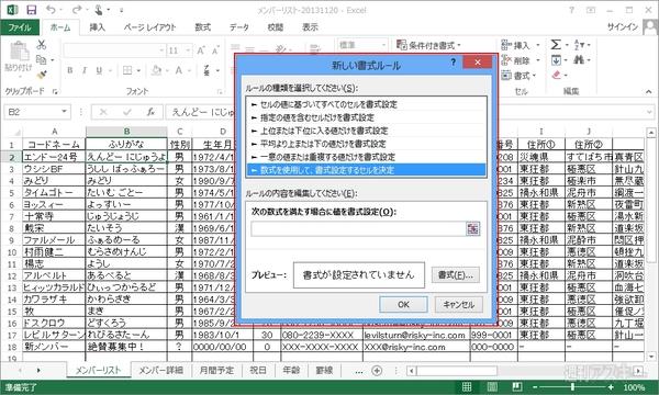
↑ In the window for creating a format rule, select “Determine a cell to set the format using mathematical formulas” for the type of rules.

↑ Set the search range.Add "$" only for the column side.

↑ Add a search keyword enclosed in double quotation.

Step3 Edit the corresponding cell format rules

↑ Set the cell format that corresponds to the conditions in the “Preview”.What can be changed is the color, size, cell background color, etc.

↑ Conditional format rule setting is completed.If you want to change the conditions, select "Edit rules" to the above setting screen.

Step4 Set multiple format rules and color the table

↑ It is also possible to set multiple formal rules.Change the search string, and add rules in which the formatting is changed accordingly.

↑ When all format rules are completed, click the “OK” button.Then, the format of the line corresponding to the conditions is automatically changed.

Step5 Applies the format to the newly entered data

↑ The conditional format is automatically applied for a conditional format.The format will be changed when the newly input data is set to the conditions set.

↑ The format is changed immediately the moment the data is entered.It is useful to save the trouble of changing the format.

As mentioned above, I have seen color coding by "fixing rows and columns" and "conditional format".Please use it for practice."Excel Dojo -Secret Society Listing Raise" is being popular in the Weekly ASCII magazine.Please check it out and enjoy Midori's great struggle!

In addition, the Office 2013 is bundled and uses the “8 -inch Windows8 tablet” that can be purchased from around 40,000 yen as Office!The mook is also on sale.From the wise operation method of 8 inch tabs to the use of Excel, it is a book filled with Gissiri.Please purchase at a bookstore or online bookstore near you.